Introduction
2024 was a year where time series zero/few shot forecasting functioality made its way into LLM architectures: Moment, TimesFM, Chonos, Moirai, and many more showed up. Those were novel models but, computationally, heavy to use. So soon the second wave of lighter models appeared incluging Tiny Time-Mixer (TTM) architecture from IBM Research. TTM can work with just 1M parameters, it supports channel correlations and exogenous signals, and handles multivariate forecasting. Let’s dive in.
You’ll find the TTM research paper here.
Architecture
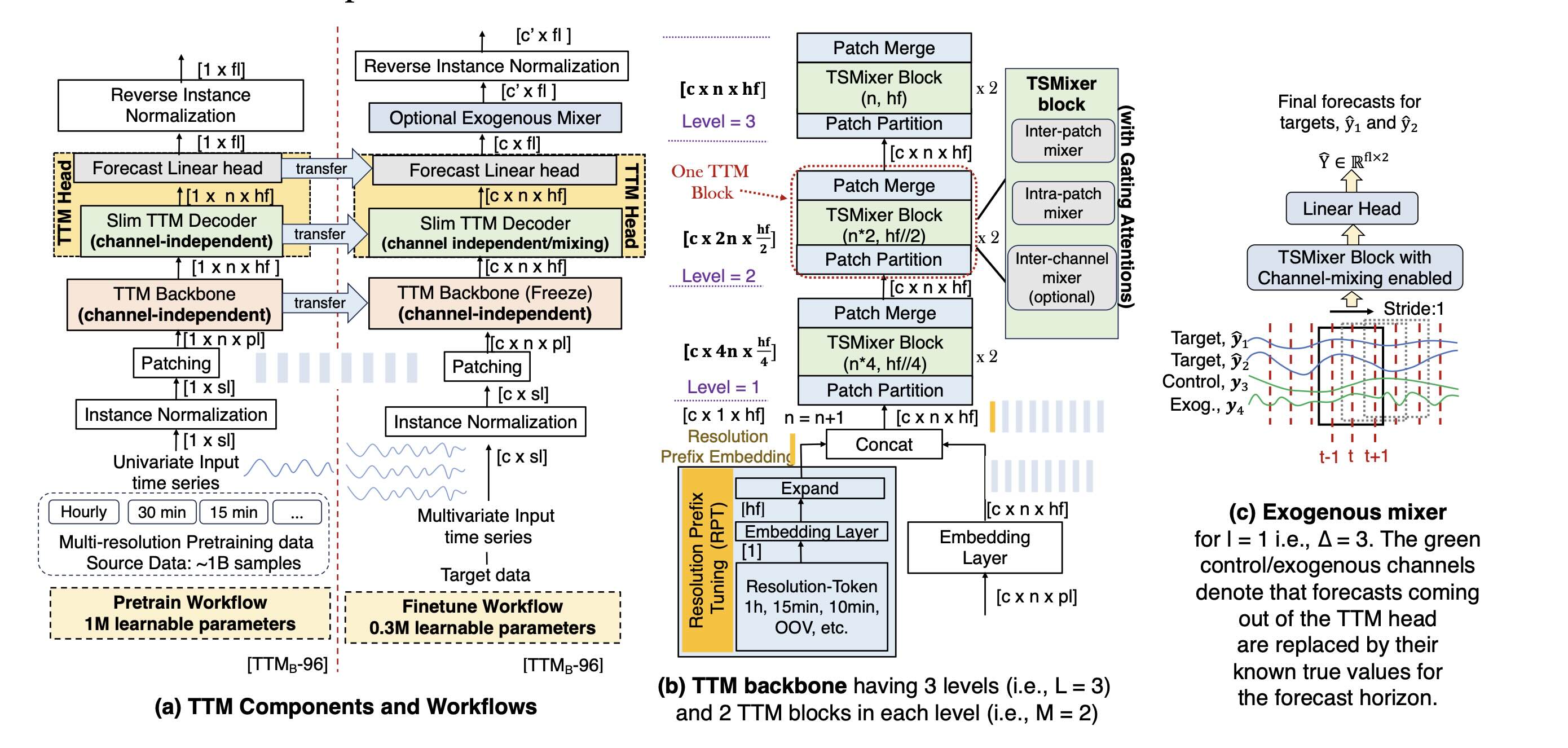
Great way to think about TTMs is like this: a powerful feature extractor + mixing network that reads a 512-point window and outputs the next 96 points in one shot. No decoder loop. No cross-attention. No auto-regressive generation. Let’s get into details.
TTM model is based on TSMixer architecture (it came originally from MLPMixer, Google, 2021). In TSMixer multi-head attention is replaced with simpler mechanism: mixing information across time and features using simple MLPs (linear layers). This solves the problem of classic self-attention being to slow for long sequences. Self-attention compares each token to every other token, this is O(n²) complexity, so those ‘classic’ attention layers scale quadratically with sequence length n. And the time series can be a very long sequences with thousands of tokens.
So we have TSMixer encoder mechanism explained above. There is no decoder side needed, the model processes a fixed-length context window of 512 points and outputs the forecast window of 96 points directly.
When it comes to pre-training/finetuning the TSMixer architecture has few nice additions to original MLPMixer: 1) adaptive patching across layers, 2)diverse resolution sampling, 3)resolution prefix tuning, 4) multi-level modeling strategy. I will focus on last one: modeling of channel correlations on many levels at once: independent singular channel patterns, cross channel patterns, global patterns. So, the TSMixer is modeling the data from many channels on 3 levels simulatneusly to give us the prediction. It’s like making a prediction having several time-series data of potentially correlated channels:
- temperature
- traffic
- energy consumption
- humidity
TTMs are modeling these on three levels simultaneously.
1B samples used in model creation comes from Monash and Libcity datasets. Monash is ~250M samples and Libcity is the rest. Monash collects time series from many areas: weather, traffic, banking, bitcoin, eletricity, and more. Libcity is about city traffic time series. IBM’s TTM models are open-sourced on huggingface, you can find more details in Training Data section here: https://huggingface.co/ibm-granite/granite-timeseries-ttm-r2
Running the model
Trying this right now - https://colab.research.google.com/github/ibm-granite/granite-tsfm/blob/main/notebooks/hfdemo/ttm_getting_started.ipynb
(notes and thoughts will come soon) This colab uses TTM-512-96 model. It means that one can take input of 512 points and make a prediction 96 points.
The notebook load ETTh2.csv, one of widely used benchmark time-series datasets and its about load levels of electrical system connected to power (electrical) transformer.
work in progress….